
This blogpost is overtaken by a better analysis by Kurt Allan, based on other analysis by Louis Kessler and information from Doug Speed that his chart was intended for a different purpose and might not apply to genetic genealogy. The result is a spreadsheet similar to the one below, but with a more normal distribution curve with 7C-9C occupying the mean. This is very good news for genetic genealogists – most of our Matches are well within a genealogy horizon. I hope to be able to post or link to Kurt’s final graphs soon.
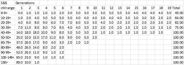
A recent discussion on the Genetic Genealogy Tips & Techniques facebook page asked about what percent of our DNA matches we should expect at various genetic distances. I’ve often wondered about this too. As I thought about it, we should be able to apply the “Speed and Balding” analysis to this question. The S&B graph shows the probability of a matching DNA segment at different generations (think cousins), for given ranges of shared DNA. See the graph at the ISOGG wiki here.
I scaled each “bucket” in this chart as best I could and put the bucket percentages in an excel spreadsheet – see below. In the Speed and Balding chart, cM ranges are along the x-axis; percentages on the y-axis; and the “generations” are shown as stacked bars (or “buckets”) for each cM range. The numbers in the body of this chart are the percentage for the cM range and Generation.
I had in my files a complete download of my AncestryDNA Matches by DNAGedcom Client from several years ago, before the Ancestry purge of 6-7cM Matches. I had 131,824 Matches and it was easy to sort by cM and determine the total number of Matches for each column (cM range) in the S&B chart. Finally I applied the S&B percentages to my breakdown of Matches to get the following chart.
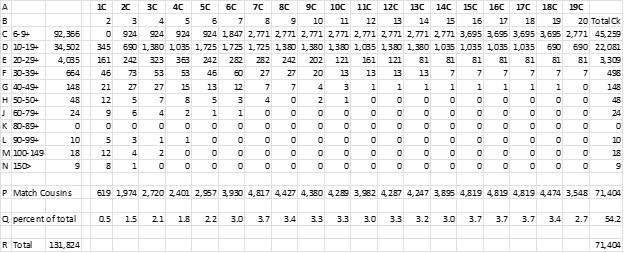
I know it’s a “squinter”, but I wanted to show the whole spreadsheet. Here are explanations of the lettered rows:
A. The cousinship which corresponds to the S&B generations back
B. Speed & Balding generations
C-N. The first column is cM range groups that correspond to the S&B chart.
C-N. The second column is the number of my Matches in each category –131,824 Total.
C-N. The next columns: multiply S&B percent by number of Matches in the cM range
P Total number of Matches for each cousinship
Q Percent of cousins vs the 131,824 Total
Key points
1. I could be off by a percent or two in my scaling of a printout of the Speed and Balding chart – but the totals are pretty close, and what I am really looking for is trends and order of magnitude.
2. Line Q, percent of total, was a lot flatter than I had expected – less than 4 percent for any cousinship. I had expected something closer to a normal distribution curve – even a long one, but with a “hump” somewhere. This indicates the two competing factors: an increasing number of cousins with each generation going back, verses a decreasing probability of a shared DNA match (above 6cM) with each generation going back.
3. There are a lot of Match-cousins to work with. Although only about half of all our Matches would be related to us out to the 19th cousin level; nevertheless, there are thousands of cousins in every cousin “bucket”.
4. In my own case I need to use judgment and temper some of these results. Both of my parents were only children, so I have no 1st Cousins. And my great grandparents did not have large families, so I also don’t have many 2C. However, I do have about 300 3C Matches and 600 4C Matches identified, so far, and there are plenty more out there (at least per Speed and Balding). And I am finding many 5C-8C Matches (but my known Tree begins to thin out after that.)
My Takeaways
1. Autosomal DNA “works” throughout a genealogy horizon for most of us.
2. The limiting factor is NOT the atDNA, it’s the genealogy – the lack of good Trees among our Matches; and the shrinking body of documentation the farther back we go.
3. When Matches Triangulate or group in Clusters, it’s often worth the effort to extend their Trees and find the Common Ancestor.
This blog post is one in a series to try and outline what you can generally expect – to put some generalized boundaries on genetic genealogy.
Anyone is welcome to use my estimate of the S&B data in the first spreadsheet, and apply it to the distribution of your own Matches. Please let me know if you see a glaring error in this process or the results.
[06D] Segment-ology: Distribution of Cousins by Jim Bartlett 20211209

Woah and wait a minute I just made a comment on another post here about the same thing – how I struggle with the logic of saying the relationships are distant when they share enough DNA to be detected by a DNA company. Here is a chart I made if you like Excel. Every single relationship category possible (with the exception of twin descendant relationships) categorized by degree and by generational separation including the percentages and shared centimorgan estimates for each degree/category. It goes back 25 generations. There is even a slider tool for finding the parent of any relationship category and you just slide the tool over until you reach the MRCA
LikeLike
Marilynn – please see my other reply to you – there is a range of possibilities for each cousinship. Jim
LikeLike
Jim,
Thanks so much for bringing this out again. I look forward to seeing what Kurt ends up with.
And for showing me up! I thought I was doing well with some 13C matches, but I must try harder.
Gives me a spur to maybe this year tackling an actuarial problem for ordinary genealogy.
LikeLike
Christopher – we are all learning at a faster pace. Jim
LikeLike
I intended to provide this link to “Revisiting Speed and Balding” by Louis Kessler’s Behold Blog. I was surprised how readable this is… not over my head like most technical articles are. https://www.beholdgenealogy.com/blog/?p=2338
LikeLike
Kurt, Thanks for the link. I’ve read all of Louis’s posts and updates and most of the links. I’m still not convinced that all the math and models are giving us a true picture that applies to our lists of Matches from the DNA companies…. I have a hard time with conclusions like 10cM shared DNA segments are largely from so many generations back. I can easily believe that a large percentage of our under 10cM Matches are False. And I know many True Match cousins are very distant. But I continue to find Matches with Common Ancestors who “fit” in my TGs and Clusters. I continue to focus on what I can do, not what I cannot do.
LikeLike
Hi Jim. This is my first blog comment in any blog ever. I have enjoyed your segment-ology blogs several times now and special thanks for this subject. I think there is value in knowing the probabilities of cousinship for any individual match of say 8 cM, or 13 cM, or 21 cM. You definitely have pointed me on the right track to doing this. I also think we need to incorporate the ISOGG “How Many Cousins Do We Have?” chart at https://isogg.org/wiki/Cousin_statistics as has previously been done by Louis Kessler. My biggest problem now with this is the large bucket sizes 6-9 and 10-19 cM. Almost all my matches fit in just those 2 buckets. I’m presently going back and duplicating Louis Kessler’s work, except with 1 cM wide buckets. I will have individual buckets for 6 cM, 7 cM, 8 cM, etc. and probabilities of cousinship associated with each of those… probably tomorrow. Today I’ll be busy helping my grandson with his AP Physics.
LikeLike
I forgot to mention… I’m also confused by Speed and Balding’s equation for mean segment length at any generation G = 2667 / (22 + (40.7 + 22.9)*G). I think I’m OK with the 22 initial chromosomes, and 40.7 recombination events for females per generation, and 22.9 per male… although I don’t know why they were added together and not averaged. I’m more confused by the 2667 total cM. I’ve been using 2798 cM total for 22 autosomes, and that does not count about 84 cM of regions not covered by DNA testing. I need to give this more thought… but maybe someone else already understands this equation.
LikeLike
Kurt, I share your confusion about the equation. I think S&B were using Mbp, vs cMs – they are roughly equal over an entire genome. I think it’s OK to use either one, just be consistent. I have to be careful with these calculations – we actually have two genomes, one from each parent – and there is a different recombination rate for each side. However, that recombination rate applies only to the full genome of, say, the mother – there will be about 40.7 recombination points added to the 22 chromosomes. BUT those recombination points only apply to the mosaic of segments already present in the two chromosomes she is recombining (each of which two chromosomes have just recently (in the previous generation) been subdivided by 40.7 and 22.9 respectively). When you look at the mosaic of many generations of “pre-existing” crossovers, the effect of the 40.7 new crossovers is hardly noticed just a few generations back – so, for me, the 36 crossover average works just fine. I would use 22+36 = 58 segments per generation per side, divided into the total Mbp or cM on a side. In order to use 40.7 and 22.9 we’d need to know the Ancestor in question and work those calculations back, generation by generation, based on the gender at each generation.
LikeLike
Kurt, I really welcome your thoughts to the world of segmentology. I view genetic genealogy as a giant Chromosome Mapping puzzle – and the puzzle pieces are our DNA segments. In one of my previous posts, I tried to highlight the difference between our own segments – all of which are True, no matter the size – and our shared DNA segments with Matches – some of which are False. Each company has a different matching algorithm that strikes a balance between lots of Matches (what genealogists want), and what percent will be False Matches (what genealogists don’t want). In general we say that above 15cM virtually all shared DNA segments are True (maybe up to 18cM at MyHeritage due to imputed values). We say the rate of False Matches increases (not a straight line) as the cM value decrease; and the 50/50 (True/False) point is roughly in the 6 to 7cM range; with ever increasing False rates below that. The S&B charts cleverly duck this issue by stating that it is based on IBD (True) Segments. But what we are given in genetic genealogy are shared DNA segments, which are not all IBD. Based on my experience over the past 8 years of Triangulation, I believe Triangulation “works” down to 7cM, because it culls out many of the smaller segments which do not Triangulate on either side. Does it cull out every False shared segment? I don’t really know – it does cull out a bunch. And the point (for me) of Triangulated Groups is that it identifies a True segment in *my* DNA, with fairly finite end points, which came from an Ancestor down to me and to most (if not all) of my DNA Matches in the TG.
With my 131,824 Matches at Ancestry, 92,366 (70% of the total) are in the 6-9.9cM buckets. If roughly half of those are False, that’s a third of my Matches. However, as a genealogist, I am still interested in cousins with paper trails and documentation (even if the DNA shared segment is false, or even if there is no matching DNA). I’m not sure how to account for the False Matches below 15cM…
I look forward to your 1cM buckets (maybe just an asterisk that some percentage will be False) I note that 96% of my Matches are in the under 20cM range. We are largely dealing with distant cousins…
Good luck with the AP Physics…
LikeLike
My comment appears to have been lost.
Do S&B give any info on the proportion of chance matches at the various levels?
LikeLike
Ian, I don’t know, but I don’t think so – there study was based on the distribution of IBD segments. So that would not include Identical by Chance (IBC). IBC is an artifact of the matching algorithms. All of our own DNA is TRUE – down as small as you want to go. The testing companies record SNPs, but do not know which side they are on. The concept is that if two people share a long enough string of SNPs, it must be an IBD shared segment from a Common Ancestor. Anecdotally, this works for segments over 15cM, but below that the algorithms may report shared segments which are IBC. So IBC is not a factor above 15cM. In the range 6cM to 15cM, I use segment Triangulation, which appears to cull out the IBC segments. But the S&B study was based on IBD segments. There are other studies/anecdotes that estimate the percent IBC – in general we use 6-7cM as roughly where the IBC/IBD ratio drops to 50/50 (using unphased data). Jim
LikeLike
Particularly interested in point #3, as testing and trees expand, so should our abilities to identify ancestor dna segment sources further back up our trees.
LikeLike
James, It is interesting. If I share a TG with a 3C, that segment, or part of it, must come from one of the 4 parents of the 3C couple – that certainly narrows the search field. Jim
LikeLike
James, I should add two points: 1) I agree with you that as testing expands, we’ll get more data to work with; and 2) one of my points in the blogpost is that we already have many Matches in a genealogical time frame – the issue is that they have no or small Trees. Even a no-Tree Match has value through Shared Matches – a tight group of Shared Matches along one Ancestral line is a strong indicator that they all share the same Common Ancestor. And this information is particularly valuable for Matches with smaller Trees – it gives us an ancestral line to look for. Jim
LikeLike
Thanks Jim, I like your characterization of “tight group”, perhaps we can get better at identifying the degree of “strong indication” that can be associated with various types of tight groups. Certainly the number of triangulating matches, but perhaps also the segment size and the extent of divergent ancestral pathways might all be contributing factors.
LikeLike