Sure it does! Triangulation is a tool to use with autosomal DNA. Let’s see how it might work:
- Does it work in grouping your shared segments?
- Does it work in culling out IBS segments?
- Does it work to define and map your ancestral segments?
- Does it work to insure that all Matches in a Triangulated Group have an IBD segment?
- Does it work in identifying Matches who all share the same Common Ancestor?
- Does it work for any size segments? – see more at: Does Triangulation Always Work?
The Big Picture
Let’s start with the Big Picture. We take an atDNA test and the company reports a list of our Matches. We can also get Matches by uploading our raw DNA data to GEDmatch. Each of the companies compares our raw DNA data to that of all the others in their database, and uses their proprietary matching algorithm to generate a list of Matches. At 23andMe, FTDNA and GEDmatch, they also provide the shared segment information (Chromosome, Start Location, End Location, cMs, and SNPs) for each shared segment. For this discussion I’m only going to be talking about segments over 7cM, just to avoid any debate about smaller segments. Each of the companies have pluses and minuses that go along with their matching algorithm, but we are going to go with the list of Matches they provide to us.
So this is the data we want to work with using the Triangulation tool.
Ancestral vs Shared segments
Please re-read “What Is a Segment?” to recall there are ancestral segments – ones you get from an ancestor – located completely on one of your chromosomes; and there are shared segments – ones that the computer algorithm determines by comparing data on both your chromosomes with data on both chromosomes of another person.
Shared segments are either IBD or not-IBD (IBS)
Most of these shared segments are IBD – meaning they come from a Common Ancestor – common to you and your Match. Some of the shared segments are IBS – meaning they don’t come from a Common Ancestor; they are segments made up by the computer algorithm. We cannot tell which is which by just looking at the one shared segment. ISOGG has a very good wiki article about IBD and non-IBD (IBS) segments. The bottoms lines are:
- Shared segments (also called matching segments or Half-Identical Regions (HIRs)) 15cM and greater are IBD virtually 100% of the time.
- Shared segments under 5cMs should generally not be used in genealogical analyses [and in this post we are not considering shared segments under 7cM].
So for this blog post we will focus on shared segments from 7cM to 15cM as reported by the companies. And note that each of these segments is either IBD or IBS.
Triangulation Criteria
For Triangulation we find three sets of shared segments which match each other. This usually means you and two Matches have shared segments which overlap at least 7cM, AND the two Matches share a segment which overlaps the same area at least 7cM. This means all three of you have the same, long string of SNPs in the same location. This is Triangulation.
Usually Triangulated Groups (TGs) include more than just you and two Matches. They may include 5, 10, 20 or more Matches. Each TG includes all of the shared segments, and these triangulated segments determine the start and end locations of the TG, such that the TG includes them all.
My Experience with Triangulated Groups
I have over 5,000 different Matches in my spreadsheet, with perhaps 6,000 separate shared segments over 7cM. As a result of the Triangulation process, these shared segments have been placed into 4 categories:
- A Triangulated Group on my Dad’s side.
- A Triangulated Group on my Mom’s side.
- An IBS group (these segments overlap, but do not match, TGs on either side)
- Undetermined as yet
The TGs above cover 90% of my 45 chromosomes, and define 340 separate TG segments on my DNA. Most of the TGs are heal-and-toe (adjacent) to each other on each chromosome, with only a few gaps. All of my shared segments either “fit” into (overlap within) one of these TGs or they are IBS (or they are undetermined).
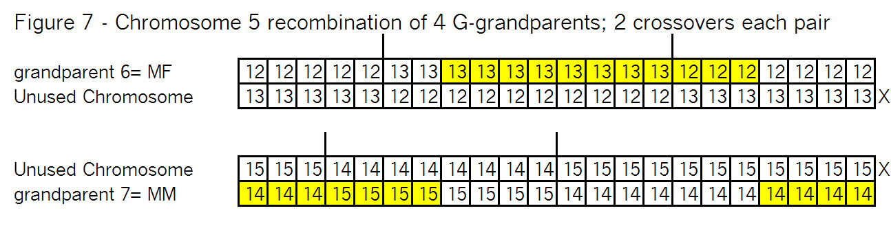
TGs Form a Chromosome Map
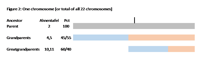
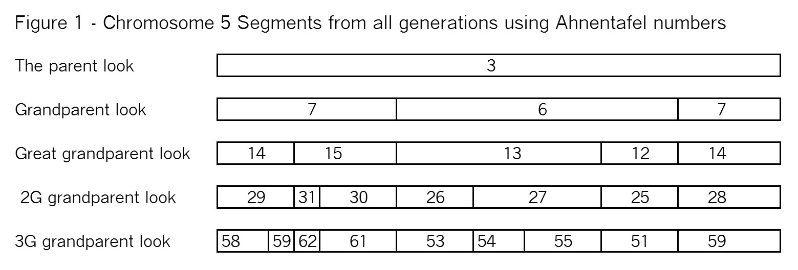
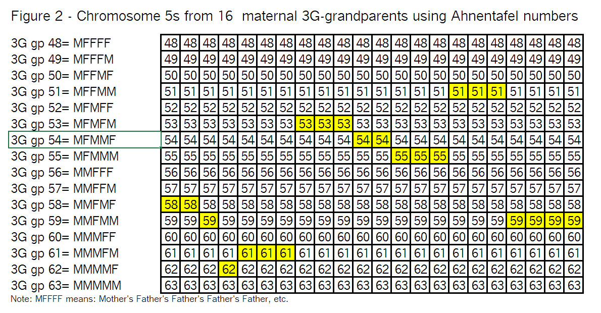
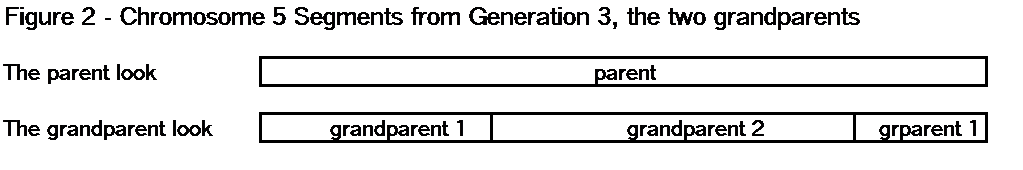
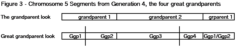
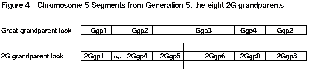
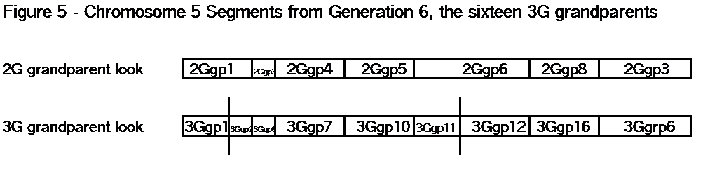
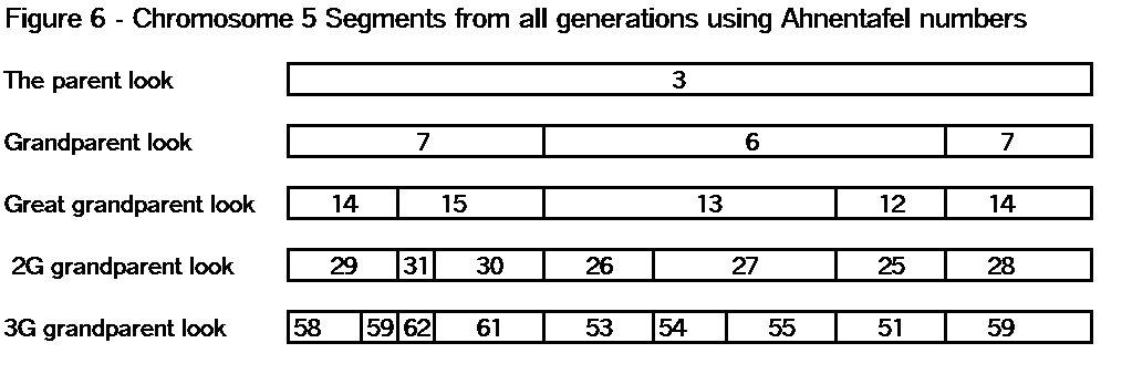
The key point here is that these TGs map my chromosomes into specific segments. Each of these specific segments comes from an Ancestor. Similarly your chromosomes are divided into specific segments, defined by crossover points from each generation. Re-read Bottom-up and Top-Down for a refresher on how crossover points and segments are formed. Within each such ancestral segment, defined by start and end locations, each of us will have a continuous string of SNPs – usually thousands of them. And each such ancestral segment comes down a specific path from a specific ancestor to us. On this point endogamy does not matter. In the bizarre extreme, all of your ancestors in one generation could be the same man and woman, but each of your ancestral segments only came from only one place in your Tree, and down one path to you.
IBS Segments
Most of your shared segments will be IBD and will form TGs. But some shared segments will overlap the segments of a TG but they won’t match any of them. On either side. These shared segments are clearly IBS. If they were IBD – from an ancestor – they would match overlapping segments in a TG.
Are All Segments in a TG IBD?
So one of the arguments for Triangulated Groups is that if three people all match each other on the same segment, the shared segments must be IBD. We have three pairs of matches, each pair with the same long string of SNPs. We have all three companies with proprietary algorithms that try to insure their Matches are IBD. We have TGs that are mapped on our chromosomes, and know that some ancestor provided that segment. It sure looks like the shared segments in these TGs have the same SNPs that our ancestors passed down to us. This is even more compelling when there are several, or more, shared segments which Triangulate and form a TG. But are we sure every segment in a TG is IBD? Read on for some possible exceptions.
Some Areas to Look Out for:
- If you have only one Match (Match1) who matches a number of your close relatives in an apparent TG: You and Match1 might share an IBS segment (based on Match1’s segment being false); and then Match1 may well match all of your close relatives who have the same ancestral segment you have. For this reason observe the caution that TGs should be formed with widely separated cousins – the wider the better. Another test is to find other Matches (not closely related to Match1 who Triangulate with you and see if they match Match1. All Matches in a TG, who overlap enough, should match each other. If they do not, then an analysis should be done to weed out any potential IBS segments.
- You match several other Matches who are closely related to each other in an apparent TG: you might have a false segment and may well match all of the Matches who share the same good ancestral segment. As in the previous paragraph, it’s important to form a TG with widely separated cousins. The test here is to look for other overlapping Matches for this segment area. If this is an IBS TG, the other Matches will not also match the Match family. Also, you do have a true ancestral segment for each area of your chromosomes. If several related Matches all match you in one segment area, and your segment is false with them, you should be able to form two other TGs (one from each parent) based on your ancestral segments compared with other Matches.
- Another argument used to debunk Triangulation, is endogamy. The theory here is that due to endogamy – some of our ancestors being the same person – the same ancestral segments are floating around and TGs may be formed with different ancestors. In theory, this is possible – in practice it is improbable. In the first place, endogamy means the two ancestors who are the same person actually had a Common Ancestor. So in fact the TG shared segment really did come from Common Ancestor, several more generations back. With each generation going back, the probability of a match is divided by 4, or 16 for the two generations involved in a first cousin endogamy. Clearly it is much more likely that our Matches in a TG are from a closer cousinship.
Also, based on my chromosome map, the ancestral segment I got for each TG is from a specific ancestor, down a specific line of descent to me. It has a specific string of SNPs that we generally think of as unique. Is it possible, in the 7-15cM range, for a Match to have exactly the same string of SNPs from a different ancestor? With random DNA almost anything is possible, but the premise of autosomal DNA is that this would be very rare. If it did occur, the shared segment would technically be IBS, because it was not identical because of descent from a Common Ancestor. But, we might have to leave the door open for this possibility.
Back to a Big Picture Thought
The number of people taking an atDNA test is about doubling every 12 months. If this continues, I’ll have 10,000 Matches, with shared segments, by this time next year; and 20,000 Matches by the end of 2017. My chromosome map has pretty much been determined (I am now focused on determining the correct Common Ancestor for each TG). A doubling of Matches means a doubling of each TG every year. The point is that if we assume 80-90% of our Match segments are IBD (I actually believe it’s closer to 95%), all of those IBD segments are being added to my existing TGs. Couple this with the fact that most of our Matches are beyond 5th cousins (I believe most of our Matches are actually 6-8th cousins, and some beyond). Even if a few of the Matches in our TGs turn out to be IBS, we are still getting a great influx of true cousins into our TGs.
So to summarize:
- Do TGs work to group your Matches? Sure! Instead of the long list of miscellaneous Matches reported by the companies, you can form Triangulated Groups. See Benefits of Triangulation.
- Do TGs work to cull out IBS segments? Sure! Many of your 7-15cM segments will not triangulate with any overlapping TG, indicating those “shared” segments are probably IBS. As noted above, not all of the IBS segments may be identified this way, but many (I think most) will. This is progress – it’s an improvement over the list you get from the companies.
- Do TGs work to define and map your ancestral segments? Absolutely! It’s hard work, but an easy mechanical process to define the TGs with start/end locations; and only a little genealogy with known relatives is needed to assign them to maternal and paternal sides.
- Do TGs work in insuring all Matches in a TG have an IBD segment? Almost all of the time, and there are ways to find and test suspicious shared segments.
- Do TGs work in insuring all the Matches in a TG share the same Common Ancestor? This is a tough one because it’s not possible to rule out some outliers. As noted above, if you carefully form the TGs, the Matches should come from the same Common Ancestor. We have lots of examples of Matches in TGs who do share the same CA. It’s very hard to prove that an IBD segment is really from a different ancestor; and I haven’t seen a single case of it so far.
Your ancestral segment in each TG does come from a specific ancestor of yours, and your cousins from that Ancestor with that segment will match you on it in that TG. As several of us have suggested, to determine the true Ancestor for a TG, you need to “walk the segment back.” This means finding cousins at various levels in each TG – a 2nd cousin, a 4th cousin, and a 6th cousin who all have the same segment and ancestral line. This is often hard, but the number of people taking an atDNA test is doubling annually, and more of these intermediate cousins will gradually show up in our Match lists and TGs.
Bottom line for me: Triangulation is a powerful tool.
11B Segment-ology: Does Triangulation Work? by Jim Bartlett 20151019