The data we get from our atDNA test is not as precise as it may appear to be. But don’t worry, it doesn’t make any difference…

Let’s start with the 3 ways we measure our DNA first (see also my blog post Measuring Segments).

Base Pairs: Our DNA has about 3.2 billion base pairs in each set of chromosomes. The Human Genome Project sequenced about 99 percent our chromosomes in 2003. Since then, scientists have continued to refine the structure and arrangement of the base pairs. Most of our atDNA tests have been based on “Build 36”, but FTDNA shifted to “Build 37” a year or so ago. Because the atDNA tests only look at about 700,000 of those base pairs, the change from Build 36 to 37 is not much different. But most of us “lost” a few Matches and “gained” a few Matches as a result. To my knowledge, 23andMe and AncestryDNA still use Build 36, as does GEDmatch. The differences are slight.

cMs: The cM is an empirical measurement. There are differences in the observed cMs for males and females over the same segment (same start and end location). An average is used because the companies just don’t know the male/female ancestry of each shared segment. Besides, an average is much easier to work with… Even the tables of averages differs by company. Here are the totals per the ISOGG/wiki (without Chr X) [1]:

23andMe                    3,537 cMs

FTDNA                       3,384 cMs

GEDmatch                  3,587 cMs

Per the CRC Research Group [2] we have very different totals of the average for males and females in the 22 autosomes:

Male                            2,809 cMs

Female                        4,782 cMs

Average                       3,795 cMs

The reason this last average is greater that the averages used by the three companies is because there are certain areas of certain chromosomes that are blocked out from atDNA testing for genealogy (see the greyed area in your chromosome browser). So the companies only take the average of the areas covered (sampled) by the SNPs.

The important point to understand is that there is a wide variation between males and females. Using an average pretty much guarantees some inaccuracy. So definitely use cMs as a guideline, but don’t split hairs or make hard and fast “rules” with the cM values we get from the testing companies

SNPs: Each of the atDNA companies use a different number of SNPs per the ISOGG/wiki Comparison Chart [3]:

23andMe                    577,382 SNPs

FTDNA                       708,092 SNPs

AncestryDNA              682,549 SNPs

Note that 23andMe now uses a somewhat lower number of SNPs, and some of them are different from the other companies. But since the SNPs are basically a sampling technique over all of our DNA, we see little differences in the shared segments now reported by 23andMe.

So the start and end location of shared segments will tend to be different depending on where the terminal SNPs are. You might think with the largest number of SNPs, FTDNA can report a more accurate shared segment, but read on…

Shared segments are determined by a proprietary algorithm at each company. I don’t know them. And even if I did, I shouldn’t report it.

When determining 700,000 or so SNPs it’s hard to get all of them read correctly. There are invariably a few miss-calls and no-calls. Each company’s algorithm has an instruction as to handle these: ignore one (or a few?) of them and report a longer shared segment; or let a miss-call or no-call break up an otherwise long segment. Based on GEDmatch examples of kits from 2 companies for the same person, each company probably does it differently.

There is no “signpost” in our DNA to indicate where an ancestral segment starts or ends. Each algorithm looks for matches between two kits, and it may well run beyond the boundaries for a particular ancestor, and in these cases pick up, random, but matching, pieces of DNA from other ancestors, which would not be IBD. This makes some shared segments look larger than they should be. A classic example is a parent-child-Match trio where the child-Match shared segment is a little larger than the parent-Match shared segment.

The algorithms may also include some shortcuts. Notice the large number of segments at FTDNA which end in “00”. It appears some of their algorithm is based on looking at blocks of 100 SNPs at a time – in this case the size of a shared segment would be rounded down to only the blocks of 100 that match. The advantage FTDNA might have because of more SNPs in total, is offset by using them in blocks.

Here is a quote from the 23andMe Family Inheritance: Advanced page: “… segments can be measured in centiMorgans or in base pairs for mapping onto the genome. 23andMe rounds the segment length to the nearest tenth of centiMorgan and segment start and end coordinates to the closest millionth base pair to reflect the uncertainty in the exact locations of the segment boundaries.” [bolding by me]

AncestryDNA states their algorithm culls out segments based on “population” phasing. They also eliminate some pile-up segments, although it’s not clear (to me anyway) what size range they consider for this culling process. This process eliminates some IBS segments, but is also eliminates some IBD segments, too.

All of the above factors, and probably more, result in the DNA data being a little different, depending on the company – we can say the data is a little fuzzy, and not quite as precise as it appears to be. With this knowledge, I’m pretty sure cMs values are not accurate to two decimal places, and shared segments are not precise to a particular base pair.

Clearly this fuzzy data leads to fuzzy segments. The statement by 23andMe is a good one – round the segment start and end locations to the nearest million base pairs.

So let’s look at all of this fuzzinessfrom the Big Picture of Chromosome Mapping with Triangulated Groups – is it significant?

Each TG is a collection of overlapping shared segments (which match each other). As far as defining a TG is concerned, the only two SNPs that count are the first one and the last one. These SNPs are often from one of the segments that overran a little – either at the start or the end location. So the TG may be a little larger than indicated – the ends of the shared segments are a little fuzzy, so the TG is a little fuzzy, too.

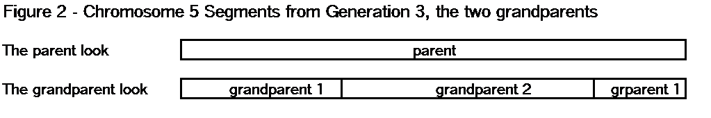
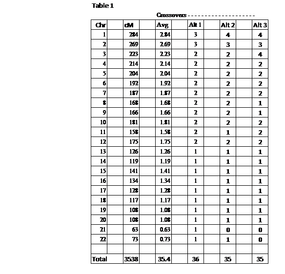
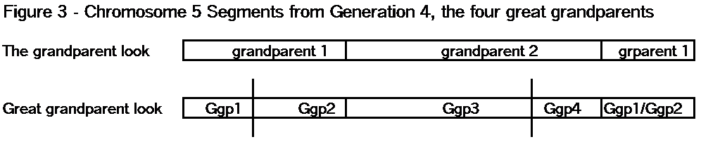
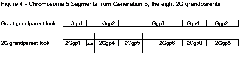
When Chromosome Mapping is complete, you should have a bunch of TGs that cover each chromosome, from one end to the other (see Segments: Bottom-Up). I often use chromosome 5 in examples because it is about 200cM, and averages about 2 crossover points per generation. In my Chromosome Map, so far, I have 9 paternal TGs and 11 maternal TGs that cover my two chromosome 5s. From the detailed data, the tips of these TGs may overlap a little. By a little I mean maybe up to 1 or even 2 Mbp. Don’t let it worry you. In the Big Picture, if you have 10 TGs with various Common Ancestors on chromosome 5, you’re doing great! You’ve won! The fact that you don’t know precisely where each shared segment or TG starts or ends, pales when you run Kitty’s Chromosome Mapper [4] and see your ancestors mapped across chromosome 5. The little fuzziness is lost in the Big Picture. When you finish a jigsaw puzzle and step back to admire the full picture, you don’t even notice the outlines of each puzzle piece. For genealogy, you have achieved your objective – notwithstanding the fuzziness.

Another clue that fuzzy data and fuzzy segments are not an issue, is that my Matches who have tested at multiple companies, still share virtually the same segments with me. The shared segments are almost never identical in start/end locations, cMs or SNP counts. However, they always show up within a few rows of each other in my sorted spreadsheet. And they always wind up in the same TG!

So if you want to make life (TGs and Mapping) easier, use Mbp for segments. And since they are just guidelines, round off cMs to the nearest whole number. It won’t hurt anything. For me, overlapping segments and cM thresholds are just guidelines to group segments, and then form TGs (see How To Triangulate)

And if, someday, you decide to tackle genes, and you need to know exactly which ancestor gave you the gene that appears to straddle two TGs (meaning two ancestors), you can reexamine that junction more carefully. You can always refine the crossover points later, if you want. But for now, spend your energies in forming the TGs and determining Common Ancestors for them! I’m curious about which ancestors gave me which genes, but I doubt I’ll ever go back once my chromosomes are properly mapped to distant ancestors – I’ll be pooped and ready to try something else…

Reference links:

[1] http://www.isogg.org/wiki/CentiMorgan

[2] http://europepmc.org/backend/ptpmcrender.fcgi?accid=PMC52322&blobtype=pdf

[3] http://www.isogg.org/wiki/Autosomal_DNA_testing_comparison_chart

[4] http://kittymunson.com/dna/ChromosomeMapper.php

03A Segmentology: Fuzzy Data, Fuzzy Segments – No Worry by Jim Bartlett 20150529

This blog post looks at the segments you got from your ancestors. It will be an effort to outline what you should expect from various ancestors – to give you an overview of how you got your segments, and how they are arranged. Your DNA is like a big jigsaw puzzle, with many different and unique pieces – this will let you see a picture that might help you solve the puzzle. Of course, your picture will be somewhat different. DNA is very random, and there is wide variation in what you actually got. Nevertheless, there are averages, and there are some rules. I hope this post will give you an understanding of the big picture, as well as some detail, and help you work with atDNA segments.

There are two ways to look at your DNA: Top-Down and Bottom-Up.

Top-Down is the way you got your DNA segments – from your distant ancestors (from the top of your Tree), down to you (at the bottom of your Tree). This Top-Down explanation often includes many ancestors and DNA segments (lots of colors in the diagrams), and can get quite complex after a very few generations. I’ll attempt a simple version of the Top-Down look in a separate blog post.

Bottom-Up tends to be the way we look at our DNA – we start with all of our own DNA and divide it into maternal and paternal sides; and then determine the segments from grandparents and Great grandparents, etc. We work from ourselves (at the bottom of our Tree), up the Tree as far as we can go. This is the “look” that will be described below.

Before we start, there are three points to make:

• We are talking about ancestral segments (see What is a segment). These are all segments you got from your ancestors.
• We are not talking about shared segments with Matches. This discussion is only about you and your ancestors and the segments from them. There will be more about shared segments in later other blog posts.
• DNA is random. This is a rough model; a general picture of our DNA segments. Please don’t get lost in the technical details or in an unusual situation. This is all about what you are likely to encounter – it’s definitely not a one-size-fits all description. Your DNA is different, but the general principles below will apply.

Before we discuss shared segments (in a later blog post), it’s important first to understand how our DNA is made up of segments from different ancestors, and generally what to expect about these segments – how they are arranged in each chromosome. This understanding of ancestral segments will help you understand shared segments later.

Three ground rules:

• This discussion will be about autosomal DNA (atDNA) – the numbered chromosomes (chromosome 1 to 22)
• This discussion will focus on one parent – Mother. The concepts apply equally to either parent.
• Examples will usually use chromosome 5.

So let’s get started…

Parents

You get many large segments from your Mother. They are exactly the size of each chromosome – because each segment is a chromosome. Your Mother gave you one of each of the 22 autosomes (chromosomes 1 to 22). In each case this is a large segment from the beginning of a chromosome (the first base pair) to the end of each chromosome (the last base pair). You probably already knew that you got one set of chromosomes from your Mother, but you may not have thought about them as very large segments. But this is all about segment-ology. You get your DNA segments from your ancestors – your Mother is an ancestor, and she gave you the ultimate segments – entire chromosomes.  See the chromosome 5 example in Figure 1.

So where did your Mother get this large segment? She got it from her parents – your two grandparents – through a process called recombination. Read on…

Recombination and Crossovers

Here is a very brief overview of recombination and crossover for genealogists:

A parent takes parts (segments) of the two chromosomes from her parents, and creates one new chromosome which she passes on to a child. Basically, when recombination occurs, a parent starts with one of their parent’s chromosomes and then shifts, or crosses over, to the other parent’s chromosome. This recombination results in two segments separated by one crossover. This process may be repeated several times on one chromosome. We’ll talk more about the probability of recombination below.

Recombination is a very complex process that is the cornerstone of life and diversity. You can google “DNA recombination” for more, but this brief summary is all you really need to know for genetic genealogy. See the Figures below to see examples of how this works.

Three important points:

• After recombination, the new chromosome is exactly the same size as each of the two chromosomes which were used to form it.
• The segments are “heel-and-toe” – that is, they are adjacent. When one segment ends, the next segment starts. There is no gap between segments.
• The crossover point marks the point between segments from two different ancestors. You change from one ancestor to another at this point. 

Grandparents

So let’s look at your maternal chromosome 5 at the grandparent level. That is chromosome 5 with segments from the two maternal grandparents. See the chromosome 5 example in Figure 2.

There is lots of information here:

• Segments from the two grandparents “fill up” the entire chromosome.
• The segments from the grandparents alternate.
• There are three segments and two crossovers (we will look more into the number of segments and crossovers below).
• There are no gaps between segments.
• These segments tend to be large, and the crossover points tend to be widely separated.
• Note: Only ancestors from grandparent 1 can contribute to the segments from grandparent 1. In other words the segments for grandparent 1 can only come from the ancestors of grandparent 1. Ditto for grandparent 2.

Crossover Points

OK – before we continue, we need to look at the realistic number of segments and crossover points we should expect in each generation. Science has found that in one generation (Mother to you, for example), there are about 35 crossover points spread out over all 22 chromosomes. In fact the cM is defined by the probability of a crossover – such that there is a probability of a crossover every 100cM. So let’s look at Table 1:

Each atDNA testing company shows a slightly different table of cMs for each chromosome. You can see a report of cM for various companies at http://www.isogg.org/wiki/CentiMorgan. Don’t get hung up on the exact numbers – it’s the overall concept that counts. The average number of crossovers is the cMs in that chromosome divided by 100. Since the number of crossovers per chromosome must be a whole number, I’ve shown several alternatives above. Although the average may be 1 or 2 or 3, possibilities may include 0 or 4 (or more sometimes). The point is that there are only a few crossovers expected for each chromosome, in one generation, and if more occur on some chromosomes, there tends to be fewer on some other chromosome. This process occurs in each generation – for instance when a parent recombines the grandparent’s chromosomes and passes a single chromosome to you. It also happens when a grandparent recombines the Great grandparent’s chromosomes and passes a single chromosome to your parent. So there are about 35 crossover points at each and every generation, and they add up, depending on which generation is under consideration. This will be described for each generation in more detail below.

Important points from the above info:

• Recombination does not “puree” the DNA into tiny pieces (segments). Recombination tends to divide each chromosome into a few segments.
• Clearly with only a few recombinations, the resulting segments in one generation will tend to be large.
• Clearly with only a few crossover points, they tend to be distributed over the chromosome.
• DNA is random, and the number of crossovers in your chromosomes may vary. If you have more than average on some chromosomes, you will probably have fewer than average on some other chromosomes.
• Regardless of the number of crossovers, or their locations, all the resulting segments on a chromosome will fill the chromosome, with adjacent segments, from one end to the other.
• When there is 0 crossover, this means there was no recombination. This means that chromosome was passed intact to the next generation. Given the probabilities in Table 1, there is a high probability that at least one of the smaller chromosomes will be passed intact with each generation.

Great Grandparents

So, given the probability that there are two additional crossovers in each generation for chromosome 5, let’s look at a probable scenario from the Great grandparent’s perspective in Figure 3.

Important information from Figure 3:

• Again, segments from the four Great grandparents “fill up” the entire chromosome.
• The “new” segments from the Great grandparents alternate; and they alternate within their respective child. That is Ggp1 and Ggp2 are parents of grandparent 1; Ggp3 and Ggp4 are parents of grandparent 2.
• There are two new crossover points (shown by large vertical lines); and the previous crossover points are still there.
• There are no gaps between segments.
• Again, these segments tend to be large, and the crossover points tend to be widely separated.
• Note: Only grandparent 1 ancestors (Ggp1 and Ggp2) can contribute within the segments from grandparent 1. In other words the segments for grandparent 1 can only come from the ancestors of grandparent 1. Ditto for grandparent 2.
• We only had two new crossover points for chromosome 5, so they could only subdivide two of the three grandparent segments. Sometimes there may be 3 crossover points, but then, sometimes there may only be one crossover point. Even with 2 crossover points, they could have both occurred within one grandparent segment. When dealing with random DNA, there are many possibilities. We used the average of 2 crossover points to paint the best overall picture. You are invited to print Figure 3 and randomly place one, two, three or four crossover points anywhere you want. If you put two, or more, crossovers in one grandparent segment, be sure to alternate the Great grandparent’s segments: Ggp1-Ggp2-Ggp1…
• Note that there is no crossover point through the last segment for grandparent 1. That means the second grandparent1 segment was passed down, intact, from one of the Great grandparents. There is a 50% probability for either one. But only for one. We sometimes refer to such a segment as a “sticky segment”, because it appears to stick together through a generation.
• We now show five, rather large, segments at this Great grandparent level of chromosome 5.
• Note that the first new crossover point divides the grandparent 1 segment into two segments, one for each parent of grandparent 1. On the other hand, the second crossover point is separating two segments from different parents of the grandparents. These two parents, labeled Ggp2 and Ggp3 are not related to each other by marriage or otherwise. So some adjacent segments may be for husband and wife; and some may be for distant, unrelated ancestors.

2Great Grandparents

OK – moving on to the next generation back – continuing our Bottom-Up look… Again, we will add two more crossover points to get Figure 4:

Important information from Figure 4:

• As always, segments from the 2G grandparents “fill up” the entire chromosome.
• The “new” segments from the 2G grandparents alternate; and they alternate within their respective child. For instance 2Ggp5 and 2Ggp6 are parents of Ggp3.
• There are two new crossover points (shown by large vertical lines); and all the previous crossover points are still there.
• There are no gaps between segments.
• Again, these segments tend to be large, and the crossover points tend to be widely separated. But in this example the first new crossover point occurs fairly close to an existing crossover point, so a relatively small segment is created for 2Ggp3. It happens… and small segments are created.
• Again, only segments from parents can contribute to a child’s segment. So 2Ggp1 is a parent of Ggp1; 2Ggp3 & 4; are parents of Ggp2; 2Ggp5 & 6 are parents of Ggp3; 2Ggp8 is a parent of Ggp4; and 2Ggp3 is a parent of Ggp2. Note that there are no segments for 2Ggp2 or 2Ggp7 shown. Those ancestors did not contribute any DNA to chromosome 5.
• Note that there are no crossover points through the first, fourth and fifth segments at the Great grandparent look. That means these Great grandparent segments were passed down, intact, from one of the 2G grandparents. There is a 50% probability for either one, and I selected one of those in each case for example. Now we have two “sticky segments” from the previous generation; and one “sticky segment”, 2Ggp3, which survived three generations.
• We now show seven, mostly rather large, segments at this 2G grandparent level of chromosome 5.
• Again, note that the first new crossover point divides a segment into the two parents.

3Great grandparents

Let’s look at one more generation – to get the hang of it – and then draw some general conclusions about what to expect.

Important information from Figure 5:

• As always, segments from the 3G grandparents “fill up” the entire chromosome.
• The “new” segments from the 3G grandparents alternate; and they alternate within their respective child. For instance 3Ggp1 and 3Ggp2 are parents of 2Ggp1.
• There are two new crossover points (shown by large vertical lines); and the previous crossover points are still there.
• There are no gaps between segments.
• Although at this generation going back (Bottom-up), these segments tend to be large, but with each generation, a few segments are split into smaller segments. Another relatively small segment has been created.
• Now there are 8of the 16 3G grandparents missing (3Ggp3, 4, 5, 8, 9, 13, 14, and 15)
• The last, 3Ggp6, segment has now survived, intact, from the 3G grandparent level down to you.
• We now show nine segments at this 3G grandparent level of chromosome 5.
• Again, note that the first new crossover point divides a segment into the two parents.

So what are the big-picture observations:

• At each generation going back, each chromosome is made up 100% by segments from that generation.
• The segments at each generation are adjacent to each other; there are no gaps.
• On, average, there are only two new crossovers at each generation. So only two segments are subdivided at each generation.
• From here on out, at each generation, most of the segments will remain the same size; and only a few will be subdivided.
• Some segments, particularly the smaller ones, will appear to be “sticky” and survive for several generations without being subdivided.
• More and more ancestors, at each generation, will drop out of the picture as you move to more distant ancestors. This applies only to the chromosome under consideration. These ancestors may well be found on other chromosomes. Because the DNA is random, many of your ancestors will be represented on some chromosomes, for many more generations.
• This should dispel the common idea that all segments are cut in half with each generation. This may be true for averages, but in practice, we found above that only a very few segments are subdivided each generation.
• “Sticky segments” are normal. In fact, in dealing with the smaller segments and comparing with a parent, you’ll often find you have virtually the same segment as your parent, or none at all. More on this in a later blog post on shared segments.
• When a husband and wife have adjacent segments, then that crossover was created in their child.
• Although this “picture” was developed for Mother, the same principles apply to the father’s side of autosomal DNA. And, of course, everyone’s version would be uniquely different. But, on a big picture level, it would be somewhat similar.
• You can use Kitty’s chromosome mapping program to show your results at any generation up to 20 ancestors. Just list the ancestors of that generation in the MRCA column. See http://kittymunson.com/dna/ChromosomeMapper.php

Final Thoughts

Remember this whole discussion is based on your ancestral segments. Your ancestral segments are defined by the crossover points. The crossover points are locked into your DNA when you were conceived. They never change. They define the picture of your segments in each of your chromosomes. They define which ancestral lines contribute to which segments on your chromosomes. We’ll talk about this more in discussions about shared segments with Matches. We don’t really see the picture of our own segments in a chromosome browser. The browser doesn’t know where your crossover points are. What we see in a chromosome browser are shared segments. By grouping and Triangulating these shared segments, we can learn where the crossover points are. Much more in future blog posts….

05A Segmentology: Segments: Bottom-Up by Jim Bartlett 20150523

Epilogue

In my spreadsheets and analysis, I use Ahnentafel numbers. They are a standard numerical code for each ancestor: I am 1; my father is 2, my mother is 3; my 4 grandparents are 4-7; etc. They offer a unique shorthand for indentifying ancestors.  Here is a summary of the chromosome 5 charts in this post, using Ahnentafel numbers for ancestors. Starting with 3 for my mother…

For autosomal DNA, segments are measured 3 ways:

base pairs (bp) – these are the individual building blocks (molecules) that form each chromosome. Over the entire set of chromosomes there are 3.2 billion base pairs. Each chromosome has from 48 to 250 million base pairs. So a segment can be defined by the Start Location and End Location. Think of base pairs as a physical picture of a segment – it’s physical length and location on a chromosome.

Example: Start at 23,500,000; End at 46,300,000

Many of us round to the closest Megabasepair (Mbp). A Mbp is 1,000,000 bp

Example: The segment is 23.5-46.3Mbp

Rounding makes these numbers much easier to read and to type. And, in my opinion, there is virtually nothing lost in accuracy. Mbp is just fine for genealogy, triangulation and chromosome mapping. If you want to do some analysis of a particular part of a segment for some scientific or medical reason, you may want to use bp. (I’ll discuss “fuzzy data” and “fuzzy segments” in a separate blog post)

centiMorgans (cM) – I think of cM as a “quality” factor, or a “genetic distance” of sorts. The cM is the best measure we have of genetic distance, but it is far from perfect. The cM is empirically derived – that is scientists have recorded many observations and put them into tables. From these tables the cM value between any two points on a chromosome (as measured by bp) can be determined. In very general terms, more is better, and the larger the cM of a shared segment, the closer the Match would be. DNA is very random, and there are wide ranges of cM vs cousinship (including much overlap).  See these references for more info [1], [2] and [3].

Example: A segment may be 15.4cM

SNPs – the single molecules (nucleotides), or base pairs, which show some amount of variation in human DNA. Most (99%) of our DNA is the same. For genealogy, we are looking for SNPs (sometimes referred to as markers) which are known to vary. The difference in our SNPs is what sets us apart. Basically each SNP can have one of 4 values: A, C, G or T. Each of the autosomal DNA testing companies uses a slightly different “chip” to determine these values, and they each effectively test a different number of SNPs – usually in the range of 600,000 to 700,000 SNPs. These are spread out over all of your chromosomes – think of them as a sampling of your DNA (a sampling of the most variable parts of your DNA). This might range from about 10,000 SNPs on the smallest chromosomes to over 58,000 on Chromosome 1.

Example: A segment may include 2,451 SNPs

Note that there is no firm correlation between these measurements. We can convert temperature measured in Centigrade to Fahrenheit because they both measure the same thing. All of the above measurements, measure different things. However, on average, there are about 100 cM for 100 Mbp

So, in summary:

A segment may be described: Chr 6: 23,500,000 to 46,300,000; 15.4cM; 2451 SNPs

A short cut description may be 6: 23.5-46.3Mbp; 15.4cM; 2451 SNPs

References:

[1] http://www.isogg.org/wiki/CentiMorgan

[2] http://en.wikipedia.org/wiki/Centimorgan

[3] http://compgen4.rutgers.edu/mapinterpolator

03 Segmentology: Measuring Segments; by Jim Bartlett 20150513

Here is a 3-step process for Triangulation: Collect, Arrange, Compare/Group.

1. Collect all the Match-segments you can. I recommend testing at all three companies (23andMe, FTDNA, and AncestryDNA), and using GEDmatch. But, wherever you test, get all of your segments into a spreadsheet. If you are using more than one company, you need to download, and then arrange, the data in the same format as your spreadsheet. Downloading/arranging is best when starting a new spreadsheet. Downloading avoids typing errors, but direct typing is sometimes easier for updates. I recommend deleting all segments under 7cM – most of them will be IBC/IBS (false segments) anyway, and even the ones which may be IBD are very difficult to confirm as such. You are much better off doing as much Triangulation as you can with segments over 7cM (or use a 10cM threshold if you wish), and then adding smaller segments back in later, if you want to analyze them. NB: Some of your closer Matches will share multiple segments with you – each segment must be entered as a separate row in your spreadsheet. The minimum requirement for a Triangulation with a spreadsheet includes columns for MatchName, Chromosome, SegmentStartLocation, SengmentEndLocation, cMs and TG. Most of us also have columns for SNPs, company, testee, TG, and any other information of interest to you. Perhaps I need a separate blog post about spreadsheets… ;>j

2. Arrange the segments by sorting the entire spreadsheet (Cntr-A) by Chromosome and Segment StartLocation. This is one sort with two levels – the Chromosome column is the first level. This puts all of your segments in order – from the first one on Chromosome 1 to the last one on Chromosome 23 (for sorting purposes I recommend changing Chromosome X to 23 or 23X so it will sort after 22). This serves the purpose of putting overlapping segments close to each other in the spreadsheet where they are easy to compare.

3. Compare/Group overlapping segments. All of these segments are shared segments with you. So with segments that overlap each other, you want to know if they match each other at this location. If so this is Triangulation. This comparison is done a little differently at each company, but the goal is the same: two segments either match each other, or they don’t (or there isn’t enough overlapping segment information to determine a match). All the Matches who match each other will form a Triangulated Group, on one chromosome – call this TG A (or any other name you want). Go through the same process with the segments who didn’t match TG A. They will often match each other and will form a second, overlapping TG, on the other chromosome – call this TG B. [Remember you have two of each numbered chromosome.] So to review, and put it all a different way: All of your segments (every row of your spreadsheet) will go into one of 4 categories:

• – TG A [the first one with segments which match each other]
• – TG B [the other, overlapping, one with segments which match each other]
• – IBC/IBS [the segments don’t match either TG A or TG B]
• – Undetermined [there are not enough segments to form both TG A and TG B and/or there isn’t enough overlapping data to determine a match.]
• NB: None of the segments in TG A should match any of the segments in TG B.

4. At GEDmatch – the comparisons are easy. Just compare two kit numbers using the one-to-one utility to see if they match each other on the appropriate segment. The ones that do are Triangulated. You may also use the Tier1 Triangulation utility or the Segment utility. I prefer using the one-to-one utility and Chrome.

5. At 23andMe you have several different utilities:

• – Family Inheritance: Advanced lets you compare up to 5 Matches at a time. You may also request a spreadsheet of all your shared segments; sort that by chromosome and SegmentStart, and check to see if two of your Matches match each other. The ones that do are Triangulated.
• – Countries of Ancestry: Sort a Match’s spreadsheet by chromosome and SegmentStart, search for your own name, and highlight the overlapping segments. The Matches on this highlighted list who are also on overlapping segments in your spreadsheet are Triangulated (the CoA spreadsheet confirms the match between two of your Matches)

6. At FTDNA it’s a little trickier, because they don’t have a utility to compare two of your Matches. So the most positive method is to contact the Matches and ask them to confirm if they match your overlapping Matches, or not. The ones that do are Triangulated. An almost-as-good alternative is to use the InCommonWith utility. Look for the 2-squigley-arrows icon next to a Match’s name, click that, and select In Common With to get a list of your Matches who also match the Match you started with. Compare that list of Matches with the list of list of Matches with overlapping segments in your spreadsheet. Matches on both lists are considered to be Triangulated. Although this is not a foolproof method, it works most of the time. And if you find three or four ICW Matches in the same TG, the odds are much closer to 100%. Remember, every segment in your spreadsheet must go in one TG or the other, or be IBC/IBS, or be undetermined. If a particular Match, in one TG, is critical to your analysis, then try hard to confirm the Triangulation by contacting the Matches.

7. AncestryDNA has no DNA analysis utilities. You need to convince your Matches to upload their raw data to GEDmatch (for free) or FTDNA (for a fee), and see the paragraphs above.

Comments to improve this blog post are welcomed.

10 Segmentology: How to Triangulate; by Jim Bartlett 20150511

I am sometimes asked if Triangulation “always” works. And with that question, there is always the follow up questions: with 15cM shared segments, 10cM segments, 7 cM segments, 5 cM segments, any size segments?

There are many things about DNA in genetic genealogy that are based on a distribution curve. And the distribution curve is based on experience. The classic example is IBD vs IBC segments. No one has reported, yet, any shared segment over 15cM that has proved to be not IBD. Very few examples exist for shared segments in the 10-15cM range. As we lower the range to 7cM, experience indicates that the percent IBD drops to about 50% range, give or take. The point is that there is a distribution curve, and we cannot say for certain that a shared segment below 15cM is IBD or not, just by the cMs.

Well, Triangulation is formed from shared segments. If we knew for a fact that the shared segments in a Triangulation were all IBD, then it would be an easy call. Given three IBD shared segments on the same segment area, from widely separated Matches, Triangulation should always work. But notice the qualifiers in that statement: three, IBD, same segment area, widely separated and should. This would be a very “tight” Triangulated Group, and we still need to say “should” because DNA is random and does not necessarily follow a set of rules like geometry.

In Triangulation we start with the shared segments reported by the various companies (23andMe, FTDNA and GEDmatch). The fact that three widely separated Matches match each other on the same segment, significantly increases the probability that the shared segments are IBD. So the IBD distribution curve based on cMs for a single shared segment, is shifted somewhat for Triangulation. Of course the question is how much.

In my experience, there have been a very few shared segments in the 10-15cM range that did not Triangulate. There are also some shared segments in the 7-10cM range that do not triangulate – the percentage goes up as you drop down to 7cM. This appears to be roughly in line with the non-IBD rate we see for shared segments. I have used a 7cM threshold for Triangulation for the past two years. I have not found any discrepancy, yet. About the end of 2014, I added shared segments in the 5-7cM range to my spreadsheet. Most of them did not Triangulate and were thus classified as IBS/IBC – this was expected. Some of them could not be categorized as there was no way to compare them (most comparisons at this level need to be made at GEDmatch). Some did Triangulate, and, so far, they have all “fit” in the TGs. A few of these have been very helpful.

I am comfortable saying Triangulation almost always works down to 5cM. The caveats include widely separated Matches, and an overlap of 5cM (estimated) for all segments. The TG “should” have one Common Ancestor. Eventually all TGs will be subdivided into even smaller TGs, and this will split the CAs between husband and wife – but that is another blog post, someday.

However, the question remains – what is the IBD distribution curve for TGs? At some point, as we reduce the cMs for shared segments in a TG, there will be IBC TGs. We still have the issue that algorithms can create IBC shared segments, so it’s reasonable to expect IBC TGs over a distribution range. There is no report I know of that addresses this distribution, yet. We may need to have completed chromosome maps for such an analysis.

11A Segmentology: Does Triangulation Always Work; Jim Bartlett 20150510

Benefits of Triangulating Autosomal DNA Shared Segments

1. Grouping – Triangulation of segments shared with your Matches will put most of them into Triangulated Groups (TGs). If nothing else, this organizes your list of shared segments.

2. Common Ancestor (CA) – all the Matches in a TG will have the same CA*. The shared DNA segment was passed down from the CA to each Match (which is why the segments match!). Each Match pair in a TG will have a Most Recent Common Ancestor (MRCA) between them. Between different Match pairs in a TG there may be different MRCAs – but all the MRCAs descend from the same CA.

3. Team synergy – all the Matches in a TG are cousins to each other; and they all have the same goal: determine the CA. They are automatically a research team. Think of the synergy of such a Team, all focused on the same goal. Each sharing their own insights and info. All working together…
4. Multiple Common Ancestors – You may have more than one Common Ancestor with a Match (it’s not uncommon with Colonial American or Ashkenazi Jewish or other endogamous populations). TGs let you sort this out. TGs help you determine which one provided the shared segment (and is thus proved by matching DNA.) When several Matches in a TG can agree on the same CA, we have genealogy triangulation. This means several widely separated cousins have the same CA, so it’s highly probable that is the correct one; and all in the TG should also have the same one.

5. Multiple Shared Segments – You may have some Matches with multiple shared segments with you. Usually, these shared segments will be from the same CA, but not necessarily. You could be related to a Match different ways, on different segments. Again, the Matches in a TG need to agree upon the correct CA, and in this way you can determine the few Matches that are related differently on multiple shared segments.

6. Eliminate false segments – the shared segments that come from a CA are called IBD (Identical By Descent). Not all of the segments identified by a company as a “matching” or “shared” segments are IBD, some are false positive matches. They were made up by the computer algorithm that searches for matching segments; and they typically include pieces from both of your parents which are not from one Ancestor. By forming TGs, there will be a few segments that overlap, but don’t match either of the two TGs for that chromosome area. These are false positives – often called Identical by Chance (IBC) or Identical by State (IBS). So TGs will identify and eliminate these segments – they are not in TGs.

7. Form “Pointers” – When a TG includes a known close cousin, the cousin provides a “Pointer”. You and the cousin have an MRCA – grandparents, great grandparents or more distant grandparents. Other Matches in the TG are usually more distant, but the CA for all of you in the TG has to be ancestral to the MRCA that you and your close cousin share. So that MRCA forms a Pointer to where the CA has to be.

8. Brick walls – as an example, let’s say you have 3 Matches in a TG: a first cousin, a fourth cousin and a distant Match. You know the MRCA with the first cousin, and quickly extend that back to the MRCA with the fourth cousin. You have a “Pointer”, but you have a Brick Wall beyond that. Working as a Team, your fourth cousin and the distant Match determine an MRCA that is one or two generations beyond (ancestral to) the MRCA you have with your fourth cousin. Very probably this MRCA (previously unknown to you), will be the parent or grandparent of the above MRCA with your fourth cousin – and you have worked through a Brick Wall.

9. Adoptee involvement – TGs are mechanically formed. No genealogy required. Adoptees can do this with several advantages. Their TGs validate your TGs (everyone in a TG should share most of the Matches). Their TGs may add additional Matches to the TG. The adoptee can analyze the Trees and genealogy data provided by the other Matches. An adoptee can serve as an arbiter, facilitator, even Team leader of a TG. The adoptee brings diversity and analysis to the TG Team. This is an excellent way for adoptees to “get involved”.

10. Mapping – TGs define each person’s chromosome map – their personal jigsaw puzzle. Each TG describes a puzzle piece. Once you’ve formed as many TGs as you can with your Match segments, you have a better picture of your map. With sufficient TGs, they will be heel-and-toe on each chromosome, even if you don’t know which side the TGs are on. Assigning TGs to a maternal or paternal side (a maternal or paternal chromosome) involves genealogy. But once TGs are assigned, they lock in the structure of your chromosome map.

11. Expanding TGs – As additional Matches are added to your Match List each week, they can usually be added to the appropriate TG fairly easily. Each new Match-segment will match (or be In Common With) several of the segment in one TG or the other in this chromosome area. If the new segment does not match either TG (usually with a segment size 7-10cM), then segment can be categorized as IBC. Also the TG boundaries will firm up.

12. TG names [extra credit] – now that you have TGs you can give each one a unique name – I recommend start with chromosome number, 01-23, add a letter, A-Z, to indicate about where on the chromosome it is; and then letters M and P, to indicate Maternal or Paternal chromosome (or A and B if you don’t know, yet). Examples: 07GM or 18BP. This can be used as a filing system, as each one will tie to a particular ancestral line for you, and all the info you collect from Matches or research will apply to this TG. Experience indicates you’ll have 400 TGs or so.

13. Crossover points [advanced topic] – the TGs define the recombination crossover points unique to your chromosomes. Using the recombination knowledge we have (roughly 1 crossover per 100cM in each generation), we can check our chromosome maps against this knowledge. So if we already see 4 alternating large blocks from grandparents on Chromosome 1, with an unknown block in the middle – we can be pretty confident that that block is from the grandparent that leaves us with 4 blocks, rather than now having 6 alternating blocks.

14. Phasing not required – No phased data is needed to form Triangulated Groups.

15. Phasing equivalent – Phasing is separating the values of 700,000 SNPs a person (usually you) got from each parent. For instance, a person’s maternal phased atDNA would match his/her mother’s DNA 100%. When you form a Triangulated Group on your maternal side, you know that the TG segment has exactly the same string of SNPs as your mother’s DNA would have for the same location. You don’t know the values of those SNPs, but you don’t really need to know. A TG is basically a phased segment.

16. Multiple Ethnicities – TGs will often pretty clearly show different ethnic groups. This is particularly true if parents are from very different admixtures (African, Ashkenazi Jewish, Melugeon, Native American, TimBukTu, etc.) We might also expect ancestries from England or Scandanavia to group differently; or ancestries from Germanna, Pennsylvania Dutch, or other enclaves, to group together. Multiple Ethnicities may even aid in assigning TGs to their respective sides.

* “All the Matches in a TG will have the same CA…”  Actually some TGs may span large segments (15cM or more). In these cases a close cousin is often involved. These TGs will actually subdivide into smaller TGs, which will have different CAs. Much more on this in later blog posts. In any case, the segments which tightly overlap each other will have a single CA. But be careful with spread out TGs – they may subdivide and have different CAs.

09 Segmentology: Benefits of Triangulation; Jim Bartlett May 2015

A DNA segment is a block, chunk, piece, string of DNA on a chromosome. It is typically determined by a start location and an end location on a chromosome. A segment refers to all the DNA in between and including the start and end locations.

We use the term segment in at least two fundamentally different ways:

1. An ancestral segment is one which is passed down from an ancestor. Ancestral segments are passed to you from your parents, who got them from their ancestors. Each of your chromosomes are made up of ancestral segments – much more on this later.
2. A shared segment is one which both you and a match have. Both you and your match have segments which are identical from start to end. Also sometimes called an HIR (Half-Identical Region). Also sometimes referred to as a matching segment. Note: a shared segment is determined by a computer algorithm – it may or may not come from a common ancestor – much more on this later.

IBD: When a shared segment comes from a common ancestor, we say it is IBD (Identical By Descent). Both you and your match have these identical segments on a chromosome because these segments came from the same ancestor.

Note that IBD shared segments are based on ancestral segments. The ancestral segment that you and/or your match received from an ancestor, may be (and often is) larger than the shared segment. What you see in the DNA match lists, reports, tables, or chromosome browsers, is the overlapping portion of your ancestral segment and your match’s ancestral segment. This overlap is the identical part that is reported as a shared segment.

 IBC: Sometimes a “shared segment” does not come from an ancestor. The computer algorithm creates the apparent shared segment from parts of the DNA which are not all from one ancestor. This can happen in your “segment”, your matches “segment”, or both. Thus, the fact that they appear to be identical to the algorithm is by chance. We refer to these segments as IBC (Identical By Chance) or IBS (Identical By State). In any case these shared segments do not exist on one chromosome for you and/or your match, and they both therefor are not IBD – much more on this later. The “shared segment” or “matching” segment is therefor IBC.